Do Foundational Models Actually Work for Forecasting?

Traditional forecasting

Every forecasting practitioner from a math/stats background knows the ritual. You get a new series, run the ADF test, differentiate, and hope that the series is stationary. You plot the ACF and PACF, count the significant lags, make a guess at p and q, run a grid search over AIC, wait, then, once you have figured out the period, you do it all over again with a seasonal component.

For the uninitiated, you can find a more in-depth explanation in the bible of forecasting: Forecasting: Principles and Practice

# Step 1: determine d via ADF + KPSS
def find_d(series, max_d=2):
    ser = series.copy()
    for d in range(max_d + 1):
        adf_p  = adfuller(ser.dropna(), autolag="AIC")[1]
        kpss_p = kpss(ser.dropna(), regression="c", nlags="auto")[1]
        if (adf_p < 0.05) and (kpss_p > 0.05):
            return d
        ser = ser.diff()
    return max_d

# Step 2: detect seasonal period from the periodogram
s = detect_season(m4_series)

# Step 3: AIC grid search over (p,q) x (P,Q)
for (p, q), (P, Q) in itertools.product(search_pq, search_PQ):
    aic = SARIMAX(data, order=(p, d, q),
                  seasonal_order=(P, D, Q, s)).fit(disp=False).aic
    ...

If you wanted to modernize your forecasting approach and follow what practitioners on Kaggle are doing, you could switch to a machine learning model like LightGBM. However, with LightGBM, you first need to engineer lag features, decide how many lags to include, add rolling statistics, and tune hyperparameters such as num_leaves, learning_rate, and subsample using tools like Optuna before you can even think of generating a single forecast.

study = optuna.create_study(direction="minimize",
                            sampler=optuna.samplers.TPESampler(seed=42))
study.optimize(objective, n_trials=40, show_progress_bar=True)
best_lgb_params = study.best_params

The problem is worse than just tedium: none of this work transfers between projects. You accumulate better instincts and reusable code snippets, but every new series forces you to restart the entire process from scratch.

Deep learning did not solve the problem

The obvious hope was that deep learning would do what it did for images and text: learn a universal representation and make the hand-crafted pipeline obsolete. It did not work out that way.

The M4 competition (2018), covering 100,000 real-world series, was the first large-scale empirical test. The winner was a hybrid ES-RNN, not a pure deep learning model, but a classical Exponential Smoothing model with an RNN on top. Pure neural methods consistently underperformed compared to statistical baselines that had been around for decades.

The M5 and M6 competitions confirmed the pattern. The use of LightGBM with careful feature engineering repeatedly beat deep learning architectures. The community largely concluded that deep learning was simply too cumbersome to train on short series, too prone to overfitting, and too sensitive to architecture choices to be worth the cost of training.

The fundamental problem was that every deep learning model still needed to be trained from scratch on each dataset. It was essentially a more expensive version of the same ritual.

What TimesFM changes

Google Research published A decoder-only foundation model for time-series forecasting in 2023. I’ve noticed the advances in transformer models when they started to creep into the industry I work in, aka banking, but only recently, while reading the paper PRAGMA: Revolut Foundation Model, did it click. The core idea is simple: pre-train a large transformer on an enormous and diverse corpus of time series data, then use it zero-shot on any new series — no hyperparameter search, no statistical tests.

TimesFM is to forecasting what GPT was to NLP: a single pre-trained model that generalises across tasks it has never seen.

This is the part that matters for practitioners. After all the machinery described above — stationarity tests, seasonal detection, AIC search, Optuna — the TimesFM inference path is:

import timesfm

tfm = timesfm.TimesFm(
    hparams=timesfm.TimesFmHparams(
        backend="torch",
        horizon_len=14,
        context_len=512,
    ),
    checkpoint=timesfm.TimesFmCheckpoint(
        huggingface_repo_id="google/timesfm-1.0-200m-pytorch"
    ),
)

point_forecast, _ = tfm.forecast(inputs=[train_data], freq=[0])

There is no fit(). The model has never seen your series. You hand it the historical values, and it returns a forecast. The entire statistical/ML ritual is replaced by a forward pass through a pre-trained network.

Running the same backtesting as SARIMA and LightGBM

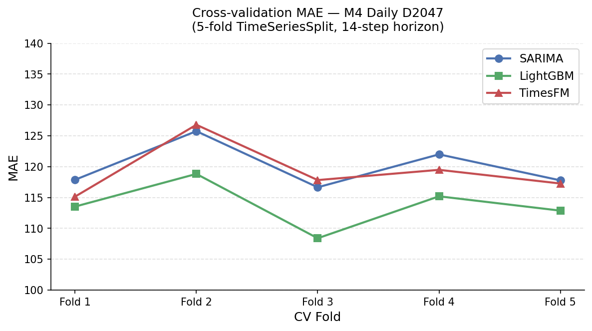
To make this a fair comparison, all three models were evaluated on M4 Daily series D2047 — 8,533 daily observations — using identical TimeSeriesSplit cross-validation with five folds and a 14-step forecast horizon.

from sklearn.model_selection import TimeSeriesSplit

n_splits  = 5
test_size = 14
tscv = TimeSeriesSplit(n_splits=n_splits, test_size=test_size)

# SARIMA: fit a new model per fold with the tuned (p,d,q)(P,D,Q,s)
for fold, (train_idx, test_idx) in enumerate(tscv.split(m4_series)):
    fit   = SARIMAX(train_data, order=best_order,
                    seasonal_order=best_sorder).fit(disp=False)
    preds = fit.forecast(steps=test_size).values

# LightGBM: train a new model per fold with Optuna-tuned params
for fold, (train_idx, test_idx) in enumerate(tscv.split(m4_series)):
    model = lgb.LGBMRegressor(**best_lgb_params)
    model.fit(X_tr, y_tr)
    # recursive prediction ...

# TimesFM: no training, same context each fold
for fold, (train_idx, test_idx) in enumerate(tscv.split(m4_series)):
    point_forecast, _ = tfm.forecast(inputs=[train_data], freq=[0])
    preds = point_forecast[0]

SARIMA requires running the full stationarity and order-selection pipeline before the loop. LightGBM requires several Optuna trials on an inner cross-validation. TimesFM requires none of that — the same three-line setup serves every fold unchanged.

The result: TimesFM achieves competitive MAE without a single line of training code, while SARIMA and LightGBM each needed a bespoke calibration pipeline just to participate.

Why this could democratise forecasting

TimesFM collapses the forecasting stack. A developer with no background in time-series statistics can load the model, pass in a dataframe, and get a probabilistic forecast within seconds.

This mirrors exactly what happened to NLP. Before the transformer era, building a production sentiment classifier for customer service calls meant curating internal transcriptions, collecting customer feedback labels, engineering linguistic features, selecting and tuning a model, and repeating this process for every new business domain or language. After GPT, it is possible to load a pre-trained model, pass in your call transcripts, and get sentiment predictions without annotation pipelines. The barrier to entry collapsed by an order of magnitude, and the volume of NLP applications in production exploded.

The limits are real

I didn’t spend five years studying statistical theory and another five as a data scientist just to watch it all get dismissed. Time series is weird in ways that GPT’s text never had to deal with. Financial returns don’t behave like energy demand. Sensor data from a factory floor look nothing like web traffic. The distribution shift between Google’s pre-training corpus and your specific problem can be absolutely massive.

Fine-tuning on domain-specific data can help close much of that gap, and Google’s own benchmarks show that even a few hundred in-domain examples significantly improve TimesFM’s accuracy. But that is still a fundamentally different burden than training SARIMA from scratch — it is adaptation, not construction.

Conclusion

Over the past decade, the pattern in machine learning has been consistent: provided that a large enough pre-training corpus is available, foundation models eventually outperform or at the very least match task-specific models trained from scratch for a fraction of the deployment cost. Text, images, audio, code — the story is always the same.

Time series proved more resistant simply because the data is messier, the frequency and domain vary wildly, and the benchmarks were designed around the assumption that every model would be trained from scratch. TimesFM, and the family of models following it, challenge this core assumption.

Whether TimesFM specifically becomes the standard, or is surpassed by the next generation of temporal foundation models, the direction is now clear. The era of bespoke per-series models is ending.